Fifty years ago, I published a paper, “Error bounds for convolutional codes and an asymptotically optimum decoding algorithm,” on the important class of convolutional codes, which is particularly effective in preventing errors in digital communication over wireless and other transmission media. The algorithm, which became labeled with my name, was a crucial step in establishing the merits as well as evaluating the performance of these codes. The paper was read and understood by only a few specialists. In the next few years, clarity was provided by two papers, the first by a colleague, G.D. Forney Jr., who introduced the trellis model, and the second by myself based on a state diagram, or Markov model.

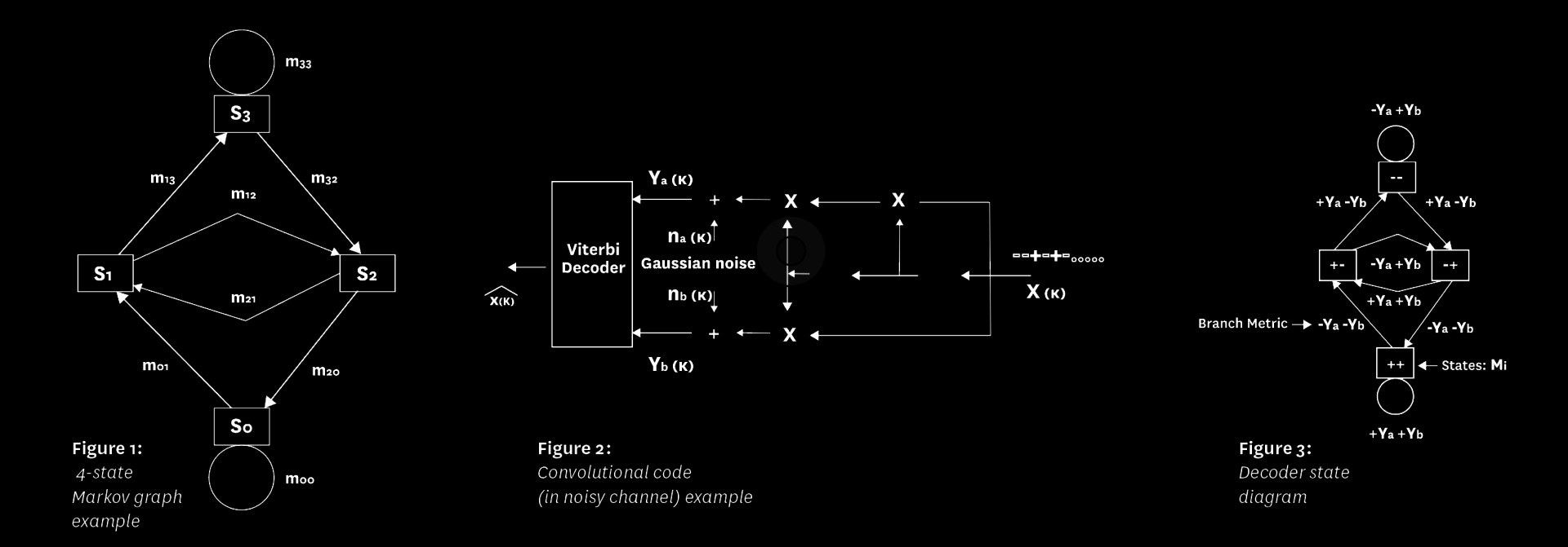
A.A. Markov was a Russian mathematician who proposed and analyzed a statistical concept regarding the relationship between terms of a sequence or, more generally, of successive events; specifically, that each term (or string of terms) or event is statistically dependent only on the previous one. To generalize, let us call terms or events simply states and describe the relationships with a state diagram (Figure 1), where the nodes represent the states and the branches a measure of the statistical relations between states.

Thus, in the example of Figure 1, each state can be followed (with non-zero probability) by only two states, one possibly a repeat of itself. The branches are labeled by a measure of the probability of the corresponding transition, known as the log-likelihood. These are called branch metrics, m_ij, where the subscripts indicate the successive connected states. The path metric (log-likelihood) is the sum of the branch metrics (log-likelihoods) of the branches it traverses in the path. We define the state metric M_j(k) as the sum of all branch metrics on the path that reaches state j at time k with the highest value. The goal of the algorithm is to find the path with the highest total path metric through the entire state diagram (i.e., starting and ending in known states). With these defining concepts and a little thought, the Viterbi algorithm follows:

M_j(k)=Max_i {M_i(k-1) + m_ij(k)}     where m_ij = -∞ if branch is missing.

In other words, the best path up to state j at time k can only be the successor of one of the best paths up to all other states at time k-1. But to select among them before maximizing we must first add the metric for the branch from state i to j (eliminating those preceding states for which there is no connection by setting the corresponding branch metric to minus infinity).

If the final state is known, the final choice of path is that which succeeded in maximizing the final state’s metric at termination. Which brings up a major issue in the implementation of the algorithm: Not only must the state metrics be computed at each stage of the process, but also the history of the path which reaches each state at each time must be stored, for ultimately this produces the answer sought. Later refinements and implementation shortcuts have removed the requirements that the initial and final states be known and even allow partial path choices to be made without waiting until the end of the process.

To examine a concrete example, we turn to Figure 2, which represents the original application for which the algorithm was proposed. Shown here is a convolutional encoder consisting of a two-stage shift register with inputs shown as + and – (in place of the traditional 1’s and 0’s) and multipliers (in place of the traditional exclusive-OR gates), but resulting in the same implementation. For redundancy, two outputs are generated for each input. Passed through a Gaussian noise channel the outputs provided to the decoder, y_a and y_b, combine according to each state-pair to form the (log-likelihood) branch metrics shown in the figure.

Practical Viterbi decoders, employed in applications such as satellite TV receivers and mobile phones, operate with convolutional codes generated by shift registers with six to eight stages. These lower the required signal-to noise ratio by better than a factor of four (6 dB), and consequently in some cellular systems proportionally increase the total number of mobiles supported in an allocated frequency band. Over the last few decades the algorithm, besides inhabiting millions of satellite receivers and billions of mobile phones, has gone viral, invading a variety of fields in both the physical and biological sciences. This has resulted from the generality of the Markov model as illustrated in Figure 1. The identification of metrics and even states in most applications is not as straightforward as for convolutional codes used over the Gaussian channel. Hence the process begins with the discovery of the Hidden Markov Model (HMM). This is the case in the adoption of the algorithm in speech recognition, genomic sequencing, search engines and many other areas.